TCGA Lung Cancer Tutorial (PyTorch Backend)
This tutorial mirrors TCGA Lung Cancer Tutorial but runs entirely on the PyTorch backend provided by Keras 3.
The code is copied from deep_lvpm.tutorial.tutorial_tcga_torch without modification, so you
can follow along step by step. The same five TCGA modalities (histology, RNA‑seq, methylation,
miRNA, and SNV) are processed with residual measurement models and connected through a five-factor
structural path model.
Prerequisites
Install deep_lvpm with the torch-* extras described on the Installation page and
set KERAS_BACKEND=torch before launching the tutorial. The bundled sample datasets under
deep_lvpm.data are used, so no external downloads are required.
1. Load the TCGA dataset and initialise the Torch backend
We begin by forcing the PyTorch backend, importing all dependencies, and loading the multi-omics training arrays.
####### Tutorial 2 #########

import os
os.environ.setdefault("KERAS_BACKEND", "torch")

import numpy as np
import torch
import torch.nn as nn
import keras
from keras import optimizers, regularizers
from importlib import resources

import deep_lvpm as DLVPM
from deep_lvpm.model import StructuralModel


with resources.as_file(resources.files("deep_lvpm.data") /
                    "Lung_multiomics_sample_train.npz") as f:
    arrays = np.load(f)
    rnaseq      = arrays["rnaseq"]
    snv         = arrays["snv"]
    methylation = arrays["methylation"]
    mirna       = arrays["mirna"]
    histo20     = arrays["histo20"]

X_arr = [histo20, rnaseq, methylation, mirna, snv]   # preserve this order!
2. Define PyTorch measurement modules
Measurement models are authored in pure torch.nn. TorchModuleLayer adapts each module so it
can run inside Keras, handling device placement and regularisation losses automatically. A small
residual block mirrors the TensorFlow tutorial.
class TorchModuleLayer(keras.layers.Layer):
    """Wrap a PyTorch nn.Module for execution inside the Keras graph."""

    def __init__(self, torch_module: nn.Module, **kwargs):
        super().__init__(**kwargs)
        self.torch_module = torch_module
        self._feature_dim: int | None = None
        self._current_device: str | None = None

    def _flatten(self, tensor: torch.Tensor) -> torch.Tensor:
        return torch.flatten(tensor, start_dim=1) if tensor.ndim > 2 else tensor

    def build(self, input_shape):
        device = torch.device("cpu")
        self.torch_module.to(device)
        feature_dim = int(input_shape[-1])
        dummy = torch.zeros((2, feature_dim), dtype=torch.float32, device=device)
        with torch.no_grad():
            features = self._flatten(self.torch_module(dummy))
        self._feature_dim = int(features.shape[-1])
        self._current_device = device.type
        super().build(input_shape)

    def call(self, inputs, training=False):
        tensor = torch.as_tensor(inputs, dtype=torch.float32)
        device = tensor.device
        if device.type == "meta":
            batch = tensor.shape[0]
            feat_dim = self._feature_dim or 1
            return torch.zeros((batch, feat_dim), dtype=tensor.dtype, device=device)
        if self._current_device != device.type:
            self.torch_module.to(device)
            self._current_device = device.type
        self.torch_module.train(bool(training))
        tensor = tensor.to(device)
        features = self._flatten(self.torch_module(tensor))
        if hasattr(self.torch_module, "regularization_loss"):
            penalty = self.torch_module.regularization_loss()
            if penalty is not None:
                self.add_loss(penalty)
        return features


class ResidualBlockModule(nn.Module):
    """Fully-connected residual block mirroring the TensorFlow implementation."""

    def __init__(
        self,
        input_dim: int,
        kernel_reg_l1: float = 0.01,
        kernel_reg_l2: float = 0.01,
        dropout_rate: float = 0.5,
    ) -> None:
        super().__init__()
        self.kernel_reg_l1 = kernel_reg_l1
        self.kernel_reg_l2 = kernel_reg_l2
        self.linear1 = nn.Linear(input_dim, input_dim)
        self.bn = nn.BatchNorm1d(input_dim)
        self.relu = nn.ReLU()
        self.linear2 = nn.Linear(input_dim, input_dim)
        self.dropout = nn.Dropout(dropout_rate)
        self._init_weights()

    def _init_weights(self) -> None:
        nn.init.eye_(self.linear1.weight)
        nn.init.eye_(self.linear2.weight)
        nn.init.zeros_(self.linear1.bias)
        nn.init.zeros_(self.linear2.bias)

    def forward(self, inputs: torch.Tensor) -> torch.Tensor:
        x = self.linear1(inputs)
        x = self.bn(x)
        x = self.relu(x)
        x = self.linear2(x)
        x = x + inputs
        x = self.dropout(x)
        return x

    def regularization_loss(self) -> torch.Tensor:
        penalty = torch.zeros((), dtype=self.linear1.weight.dtype, device=self.linear1.weight.device)
        if self.kernel_reg_l1:
            penalty = penalty + self.kernel_reg_l1 * (
                torch.sum(torch.abs(self.linear1.weight)) + torch.sum(torch.abs(self.linear2.weight))
            )
        if self.kernel_reg_l2:
            penalty = penalty + self.kernel_reg_l2 * (
                torch.sum(self.linear1.weight ** 2) + torch.sum(self.linear2.weight ** 2)
            )
        return penalty


def residual_block(
    input_dim: int,
    kernel_reg_l1: float = 0.01,
    kernel_reg_l2: float = 0.01,
    dropout_rate: float = 0.5,
    name: str = "residual_block"
) -> keras.Model:
    inputs = keras.Input(shape=(input_dim,), name=f"{name}_in")
    module = ResidualBlockModule(
        input_dim=input_dim,
        kernel_reg_l1=kernel_reg_l1,
        kernel_reg_l2=kernel_reg_l2,
        dropout_rate=dropout_rate,
    )
    outputs = TorchModuleLayer(module, name=f"{name}_torch")(inputs)
    return keras.Model(inputs=inputs, outputs=outputs, name=name)


model_list = [
    residual_block(histo20.shape[1], name="histo20_enc"),
    residual_block(rnaseq.shape[1],  name="rnaseq_enc"),
    residual_block(methylation.shape[1], name="meth_enc"),
    residual_block(mirna.shape[1],   name="mirna_enc"),
    residual_block(snv.shape[1],     name="snv_enc"),
]
3. Define the structural path and schedules
We keep the same five-factor adjacency matrix and learning-rate schedule used in the TensorFlow
tutorial. tot_num records the sample count for internal normalisation.
ndims = 5        # number of latent factors

Path = np.array(
    [
        [0, 1, 0, 0, 0],
        [1, 0, 1, 1, 1],
        [0, 1, 0, 0, 0],
        [0, 1, 0, 0, 0],
        [0, 1, 0, 0, 0],
    ],
    dtype="float32",
)

batch_size  = 256
epochs      = 300
total_steps = int(rnaseq.shape[0] / batch_size) * epochs

init_lr, final_lr = 1e-4, 1e-5

lr_schedule = optimizers.schedules.ExponentialDecay(
    initial_learning_rate=init_lr,
    decay_steps=total_steps,
    decay_rate=final_lr / init_lr,
    staircase=False
)

tot_num = rnaseq.shape[0] ## This is the total number of samples under analysis and is needed by DLVPM
4. Build and compile the StructuralModel
The StructuralModel receives the path matrix, measurement models, projection regularisers, and the standard optimiser list—one Adam instance per view.
regularizer_list = [regularizers.L1L2(l1=0.001, l2=0.001),regularizers.L1L2(l1=0.001, l2=0.001),regularizers.L1L2(l1=0.001, l2=0.001),regularizers.L1L2(l1=0.001, l2=0.001),regularizers.L1L2(l1=0.001, l2=0.001)] ## These regularizers are applied to the final "projection" layer of the DLVPM model, used internally

DLVPM_Structural_instance = StructuralModel(Path, model_list, regularizer_list, tot_num, ndims, momentum=0.95,epsilon=0.001, orthogonalization='Moore-Penrose', train_DLV =True)

opt_list = [keras.optimizers.Adam(learning_rate=lr_schedule),keras.optimizers.Adam(learning_rate=lr_schedule),keras.optimizers.Adam(learning_rate=lr_schedule),keras.optimizers.Adam(learning_rate=lr_schedule),keras.optimizers.Adam(learning_rate=lr_schedule)]
DLVPM_Structural_instance.compile(optimizer=opt_list)
5. Train and evaluate on the training cohort
Training uses the usual fit call, and evaluate reports the mean correlation metric across
connected modalities.
DLVPM_Structural_instance.fit(X_arr, batch_size=batch_size, epochs=epochs,verbose=True)
mean_corr = DLVPM_Structural_instance.evaluate(X_arr)

print('The mean correlation between data-types connected by the path model is r=' + str(mean_corr[1]))
6. Evaluate and analyse the test cohort
Load the held-out test arrays, compute the evaluation metrics, and inspect the latent correlations
via predict.
with resources.as_file(resources.files("deep_lvpm.data") /
                    "Lung_multiomics_sample_test.npz") as f:
    arrays = np.load(f)
    rnaseq_test      = arrays["rnaseq"]
    snv_test         = arrays["snv"]
    methylation_test = arrays["methylation"]
    mirna_test       = arrays["mirna"]
    histo20_test     = arrays["histo20"]

X_arr_test = [histo20_test, rnaseq_test, methylation_test, mirna_test, snv_test]   # Here, is the full test dataset list
mean_corr_test = DLVPM_Structural_instance.evaluate(X_arr_test)

print('The mean correlation between data-types connected by the path model is r=' + str(mean_corr_test[1]))

test_DLVs = DLVPM_Structural_instance.predict(X_arr_test) ## Here, we obtain the full set of test_DLVs

## Associations between the first set of DLVs are:
print(np.corrcoef(test_DLVs[:,0,:].T))
## Associations between the second set of DLVs are:
print(np.corrcoef(test_DLVs[:,1,:].T))
7. Visualise cross‑modal correlations
DLVPM can summarise cross‑modal relationships per latent factor as chord diagrams. For each DLV,
we compute a correlation matrix across modalities and render one panel. Nodes are the data types;
edge thickness and opacity scale with |r|; edges below min_corr are hidden. Optionally, label
edges with their correlation values.
# One correlation matrix per latent factor (DLV1, DLV2, ...)
corr_mat = DLVPM_Structural_instance.calculate_corrmat(test_DLVs)

from deep_lvpm.plot import plot_correlation_chord_row

data_names = ["Histology", "RNASeq", "miRNASeq", "Methylation", "SNVs"]

fig, ax = plot_correlation_chord_row(
    corr_mat,
    data_names,
    min_corr=0.0,
    node_cmap_name="Pastel1",
    figure_title=(
        "Correlation Plots Between Omics and Imaging Data Types in Lung Cancer"
    ),
    show_edge_labels=True,
    dpi=300,
    show=True,
)
Increase min_corr (e.g. 0.2) to focus on the strongest links.
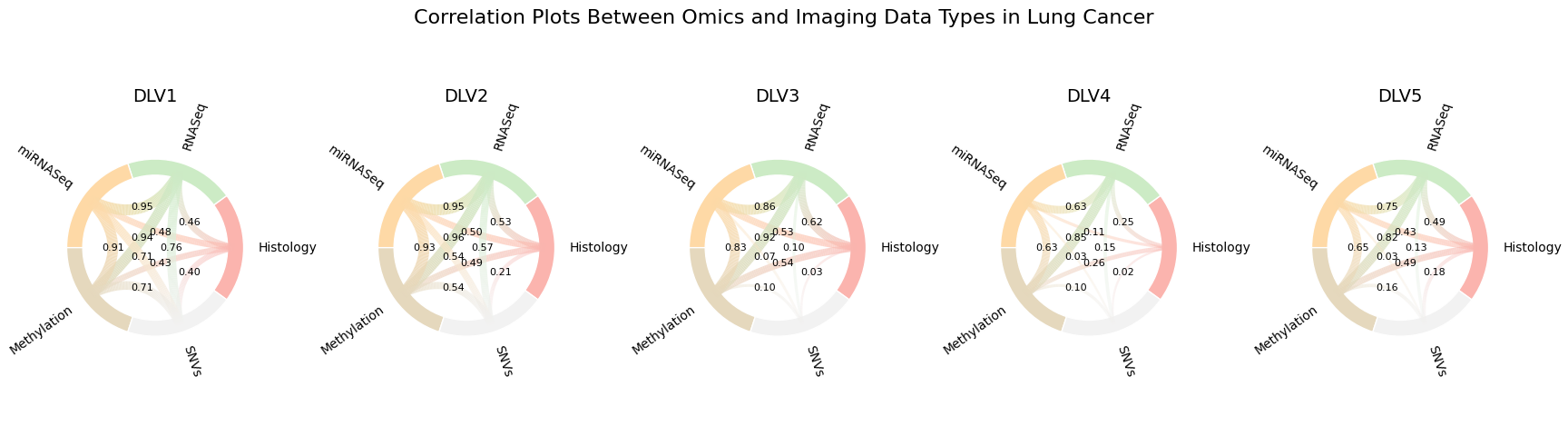
Example output from plot_correlation_chord_row. Each panel corresponds to a latent
factor (DLV). Nodes are modalities; edge thickness/opacity encode |r| between modalities
for that DLV. Labels can be toggled with show_edge_labels.
8. Save the PyTorch-backed StructuralModel
Persist the trained StructuralModel using the .keras format (which preserves both TensorFlow and
PyTorch weights + custom layers).
DLVPM_Structural_instance.save("/path/to/output_folder/DLVPM_Model.keras")
The PyTorch backend delivers parity with the TensorFlow example while letting you integrate PyTorch-native measurement modules into StructuralModel.