TCGA Lung Cancer Tutorial

This tutorial demonstrates how to use DLVPM to integrate multiple data types in a lung cancer dataset derived from The Cancer Genome Atlas (TCGA). In this example we link five different modalities: histological image features, RNA‑seq, methylation, miRNA and somatic mutation data. Each view is encoded by a small residual fully connected network and connected via a five‑factor structural path model.

Prerequisites

Ensure that deep_lvpm is installed as described on the Installation page. The tutorial uses the small sample datasets bundled with the package under deep_lvpm.data and can be run on CPU.

1. Load the multi‑omics dataset

We start by importing the necessary dependencies and loading the training data. The data files are packaged as NumPy archives inside the deep_lvpm.data module.

import os
os.environ["KERAS_BACKEND"] = "tensorflow"

import numpy as np
import tensorflow as tf
import keras
from keras import layers, regularizers, optimizers
from importlib import resources

import deep_lvpm as DLVPM
from deep_lvpm.model import StructuralModel

tf.config.run_functions_eagerly(False)   # keep graph mode for performance

with resources.as_file(resources.files("deep_lvpm.data") /
                    "Lung_multiomics_sample_train.npz") as f:
    arrays = np.load(f)
    rnaseq      = arrays["rnaseq"]
    snv         = arrays["snv"]
    methylation = arrays["methylation"]
    mirna       = arrays["mirna"]
    histo20     = arrays["histo20"]

X_arr = [histo20, rnaseq, methylation, mirna, snv]   # preserve this order!

2. Define measurement models

Each data type is processed by a simple fully connected residual block. You can experiment with different architectures or hyperparameters.

def residual_block(
        input_dim: int,
        kernel_reg_l1: float = 0.01,
        kernel_reg_l2: float = 0.01,
        dropout_rate: float = 0.5,
        name: str = "residual_block"
    ) -> keras.Model:
    """
    Builds a simple fully-connected residual block.

    Parameters
    ----------
    input_dim : int
        Number of features in the (flat) input vector.
    kernel_reg_l1 : float, optional
        L1 regularisation factor for dense layers (default 0.01).
    kernel_reg_l2 : float, optional
        L2 regularisation factor for dense layers (default 0.01).
    dropout_rate : float, optional
        Drop-out probability applied after the residual connection (default 0.5).
    name : str, optional
        Name for the returned `tf.keras.Model`.

    Returns
    -------
    tf.keras.Model
        A Keras `Model` representing the residual block.
    """
    # -------- input --------
    inputs = keras.Input(shape=(input_dim,), name=f"{name}_in")

    # -------- first linear projection --------
    x = layers.Dense(
        input_dim,
        activation="linear",
        kernel_initializer=keras.initializers.Identity(),
        kernel_regularizer=keras.regularizers.l1_l2(
            l1=kernel_reg_l1, l2=kernel_reg_l2
        ),
        name=f"{name}_dense1",
    )(inputs)

    # -------- normalise & non-linear activation --------
    x = layers.BatchNormalization(name=f"{name}_bn")(x)
    x = layers.ReLU(name=f"{name}_relu")(x)

    # -------- second linear projection --------
    x = layers.Dense(
        input_dim,
        activation="linear",
        kernel_initializer=keras.initializers.Identity(),
        kernel_regularizer=keras.regularizers.l1_l2(
            l1=kernel_reg_l1, l2=kernel_reg_l2
        ),
        name=f"{name}_dense2",
    )(x)

    # -------- residual connection --------
    x = layers.Add(name=f"{name}_add")([inputs, x])

    # -------- optional regularisation --------
    x = layers.Dropout(dropout_rate, name=f"{name}_drop")(x)

    # -------- wrap into a model --------
    return keras.Model(inputs=inputs, outputs=x, name=name)


model_list = [
    residual_block(histo20.shape[1], name="histo20_enc"),
    residual_block(rnaseq.shape[1],  name="rnaseq_enc"),
    residual_block(methylation.shape[1], name="meth_enc"),
    residual_block(mirna.shape[1],   name="mirna_enc"),
    residual_block(snv.shape[1],     name="snv_enc"),
]

3. Specify the structural path matrix

For this example we use a five‑factor model with asymmetric paths. The matrix below defines which latent factors influence each other.

ndims = 5        # number of latent factors

Path = np.array(
    [
        [0, 1, 0, 0, 0],
        [1, 0, 1, 1, 1],
        [0, 1, 0, 0, 0],
        [0, 1, 0, 0, 0],
        [0, 1, 0, 0, 0],
    ],
    dtype="float32",
)

batch_size  = 256
epochs      = 300
total_steps = int(rnaseq.shape[0] / batch_size) * epochs

init_lr, final_lr = 1e-4, 1e-5

lr_schedule = optimizers.schedules.ExponentialDecay(
    initial_learning_rate=init_lr,
    decay_steps=total_steps,
    decay_rate=final_lr / init_lr,
    staircase=False
)

tot_num = rnaseq.shape[0] ## This is the total number of samples under analysis and is needed by DLVPM

4. Build and compile the model

We create a StructuralModel instance and provide regularisers for the projection layers. We then compile it with a list of optimisers, one per view.

from keras import regularizers

regularizer_list = [regularizers.L1L2(l1=0.001, l2=0.001),regularizers.L1L2(l1=0.001, l2=0.001),regularizers.L1L2(l1=0.001, l2=0.001),regularizers.L1L2(l1=0.001, l2=0.001),regularizers.L1L2(l1=0.001, l2=0.001)] ## These regularizers are applied to the final "projection" layer of the DLVPM model, used internally

DLVPM_Structural_instance = StructuralModel(Path, model_list, regularizer_list, tot_num, ndims, momentum=0.95,epsilon=0.001, orthogonalization='Moore-Penrose', train_DLV =True)

opt_list = [keras.optimizers.Adam(learning_rate=lr_schedule),keras.optimizers.Adam(learning_rate=lr_schedule),keras.optimizers.Adam(learning_rate=lr_schedule),keras.optimizers.Adam(learning_rate=lr_schedule),keras.optimizers.Adam(learning_rate=lr_schedule)]
DLVPM_Structural_instance.compile(optimizer=opt_list)

5. Train and evaluate

Training proceeds with the standard Keras fit interface. The evaluate method returns both the mean squared error and the mean correlation between connected data types.

DLVPM_Structural_instance.fit(X_arr, batch_size=batch_size, epochs=epochs,verbose=True)
mean_corr = DLVPM_Structural_instance.evaluate(X_arr)

print('The mean correlation between data-types connected by the path model is r=' + str(mean_corr[1]))

6. Evaluate on the test set

We load the separate test dataset and compute the mean correlation of the learned DLVs.

with resources.as_file(resources.files("deep_lvpm.data") /
                    "Lung_multiomics_sample_test.npz") as f:
    arrays = np.load(f)
    rnaseq_test      = arrays["rnaseq"]
    snv_test         = arrays["snv"]
    methylation_test = arrays["methylation"]
    mirna_test       = arrays["mirna"]
    histo20_test     = arrays["histo20"]

X_arr_test = [histo20_test, rnaseq_test, methylation_test, mirna_test, snv_test]   # Here, is the full test dataset list
mean_corr_test = DLVPM_Structural_instance.evaluate(X_arr_test)

print('The mean correlation between data-types connected by the path model is r=' + str(mean_corr_test[1]))

7. Inspect the learned latent variables

To extract the latent factors for each view, call predict. This returns a tensor with shape (n_samples, ndims, n_views).

test_DLVs = DLVPM_Structural_instance.predict(X_arr_test) ## Here, we obtain the full set of test_DLVs

## Associations between the first set of DLVs are:
print(np.corrcoef(test_DLVs[:,0,:].T))
## Associations between the second set of DLVs are:
print(np.corrcoef(test_DLVs[:,1,:].T))

8. Visualise cross‑modal correlations

To understand how each latent factor relates the modalities to one another, compute a per‑factor correlation matrix and render a row of chord diagrams—one panel per DLV. Nodes are modalities; edge thickness and opacity encode correlation strength (|r|). Edges below min_corr are hidden; optional numeric edge labels show the exact r.

# Correlation matrices across modalities for each latent factor (DLV1, DLV2, ...)
corr_mat = DLVPM_Structural_instance.calculate_corrmat(test_DLVs)

from deep_lvpm.plot import plot_correlation_chord_row

data_names = ["Histology", "RNASeq", "miRNASeq", "Methylation", "SNVs"]

fig, ax = plot_correlation_chord_row(
    corr_mat,
    data_names,
    min_corr=0.0,                 # filter weaker links to reduce clutter
    node_cmap_name="Pastel1",     # pastel node colours
    figure_title=(
        "Correlation Plots Between Omics and Imaging Data Types in Lung Cancer"
    ),
    show_edge_labels=True,
    dpi=300,
    show=True,
)

Try increasing min_corr (e.g. 0.2 or 0.3) to emphasise the strongest cross‑modal associations.

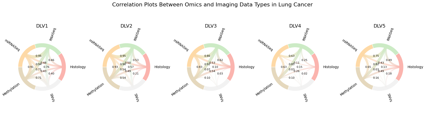
Example output from plot_correlation_chord_row. Each panel corresponds to a latent factor (DLV). Nodes are modalities; edge thickness/opacity encode |r| between modalities for that DLV. Labels can be toggled with show_edge_labels.

9. Save the model

Finally, save your trained model to disk in the .keras format:

DLVPM_Structural_instance.save("/path/to/output_folder/DLVPM_Model.keras")

This tutorial illustrates how DLVPM can be applied to real multi‑omics data. You can extend this example by changing the measurement models, experimenting with different regularisation schemes, or altering the structural path matrix to test different hypotheses about cross‑modal relationships.

If this deep dive was useful, please star the repository—community support signals that DLVPM matters and helps us justify the time invested in future improvements.